Basic Concepts

Quantum Circuits

Quantum computation involves the application of quantum operations to some qubits. A convenient way to represent this sequence of operations is to use a quantum circuit.

Let's start with an example.

The first step is to import Snowflurry:

using Snowflurry

We can then create an empty QuantumCircuit by specifying the largest qubit index (qubit_count) and the number of classical bits (bit_count):

c = QuantumCircuit(qubit_count = 2, bit_count = 2)
# output
Quantum Circuit Object:
   qubit_count: 2 
   bit_count: 2
q[1]:
     
q[2]:
     

In most cases, it can be assumed that qubit_count is equal to the number of qubits in the circuit. See Circuit Transpilation for more details about the relationship between the largest qubit index and the number of qubits. The classical bits (or result bits) form a classical register, where each bit stores the output of a Readout operation on a particular qubit.

The bit_count parameter is optional. The bit_count is set to the same value as the qubit_count if the bit_count is not provided:

c = QuantumCircuit(qubit_count = 2)
# output
Quantum Circuit Object:
   qubit_count: 2 
   bit_count: 2
q[1]:
     
q[2]:
     

We can visualize a QuantumCircuit object at any point by printing it:

print(c)
# output
Quantum Circuit Object:
   qubit_count: 2 
   bit_count: 2
q[1]:
     
q[2]:
     

Our circuit contains no quantum operations and it looks empty! Let's add some!

Quantum Gates

Unitary quantum operations are commonly called quantum logic gates or simply gates. These gates can be categorized as single-qubit gates, two-qubit gates or multi-qubit gates.

Let's start by adding a single-qubit gate called a Hadamard gate to our circuit, c. The Hadamard gate, $H$, is one of the most common gates since it allows us to create the following state:

\[H \left| 0 \right\rangle = \frac{1}{\sqrt{2}}\left(\left|0\right\rangle + \left|1\right\rangle \right).\]

This state is an equal superposition of the basis states $|0\rangle$ and $|1\rangle$. It allows us to exploit quantum parallelism (i.e. perform operations on multiple basis states simultaneously)!

We construct a Hadamard gate that operates on qubit 1 by calling the hadamard() function with the parameter target set to 1. We add the gate to our circuit c by calling the push! function:

push!(c, hadamard(1))
# output
Quantum Circuit Object:
   qubit_count: 2 
   bit_count: 2
q[1]:──H──
          
q[2]:─────

Note the exclamation mark at the end of push!. This indicates that we have called a mutating function that modifies at least the first argument. In this case, it updates our circuit c.

If we now print circuit c, we will see the following output:

print(c)
# output
Quantum Circuit Object:
   qubit_count: 2 
   bit_count: 2
q[1]:──H──
          
q[2]:─────

Let's now entangle our qubits. We can achieve this with a control_x gate. This is a two-qubit gate which is also known as a CNOT gate. We set the first argument of the control_x function to 1 and the second argument to 2. This indicates that qubit 1 is the control_qubit while qubit 2 is the target_qubit. This means that a bit flip, sigma_x, is applied to qubit 2 if qubit 1 is in state $|1\rangle$. Qubit 2 remains unchanged if qubit 1 is in state $|0\rangle$.

Let's add our CNOT gate to our circuit c:

push!(c, control_x(1, 2))
# output
Quantum Circuit Object:
   qubit_count: 2 
   bit_count: 2 
q[1]:──H────*──
            |  
q[2]:───────X──

Voilà! We just used Snowflurry to create a quantum circuit that exploits quantum parallelism and entanglement. The circuit places our two-qubit register in the maximally-entangled quantum state

\[|\psi\rangle = \frac{1}{\sqrt{2}}\left(\left|00\right\rangle+\left|11\right\rangle\right).\]

This state is one of the four celebrated Bell states, which are also known as the EPR states. These states do not have classical counterparts. They form building blocks for many interesting concepts in quantum computing and quantum communication.

Circuit Simulations

We can verify that our circuit performs as expected by simulating it on our local machine:

simulate(c)
# output
4-element Ket{ComplexF64}:
0.7071067811865475 + 0.0im
0.0 + 0.0im
0.0 + 0.0im
0.7071067811865475 + 0.0im

The output of the simulate() function is a Ket object. A Ket is a complex vector that represents the state of a quantum object such as our two-qubit system. This state is also known as a wave function.

Histograms

In the previous section, we used the simulate function to obtain the state of a two-qubit register after applying our circuit, c. However, in the real world, we cannot directly determine the state of a quantum register. Rather, we need to execute the quantum circuit several times on a quantum processor and measure the state of the qubits after every circuit execution. Each circuit execution is known as a shot. The result of each shot is a bit string that tells us the outcome of the measurements on every qubit. For instance, the bit string 01 indicates that qubit 1 was in state $\left|0\right\rangle$ after the measurement while qubit 2 was in state $\left|1\right\rangle$. The probability of obtaining a particular bit string depends on the state of our quantum register.

We can also mimic this behavior using a simulator. This can be achieved by calling the plot_histogram function from the SnowflurryPlots library. For example, we can generate a histogram that shows the measurement output distribution after running the circuit c for a given number of shots, let's say 100 times, on a quantum computer simulator.

Let's generate a histogram for our circuit:

using SnowflurryPlots
push!(c, readout(1, 1), readout(2, 2))
plot_histogram(c, 100)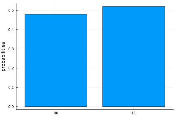

In the next tutorial, we will discuss how to run our quantum circuit on a virtual quantum processor.